Science Brief: Pulse Azimuth Clustering
The pulse azimuth effect adds an interesting dimension to the analysis, in that it uses pairs of magnetometer time series to measure the peak amplitude ratio (azimuth), that each pulse exhibits in orthogonal axes. Classically, the definition of ‘azimuth’ has been stated to be “the horizontal direction of a compass bearing.” Therefore in a site containing three orthogonal axes, North, East, and Vertical, the two horizontal North/East axes are used for azimuth evaluations.
But the peak amplitude ratio detector described here can work almost as effectively in the two vertical planes: North/Vertical; and East/Vertical also. At first, it was not a measure of the angle from the site to the epicenter or even hypocenter, but rather a more discriminative way to evaluate the pulses.
An important concept is that the pulse waveforms are unipolar, meaning that they are not like many other magnetometer signals that oscillate and decay around a zero center. The unipolar nature and large amplitude of these pulses allows one to go beyond simple peak amplitude ratios, and take instead a point-by-point measure of the amplitude ratio over the length of the pulse.
Other researchers have treated the vertical channel using the Polarization Ratio concept, eg: Hayawaka (2007) where the local signal is expected to produce more pronounced increases in the vertical coil than in the horizontal coils. In both of the channel histories studied here however, it is shown below that despite possible association with the steep angle to a hypocenter, more energy appeared in the horizontal coils than in the vertical. If the signals are originating from subsurface near a hypocenter, then the idea of evanescent propagation like Grimalsky (2003), or an analog to the seismic “head wave” discussed in Stein (2003) that occurs at interfaces between layers of differing indices of refraction might be a useful framework for discussing them.
These horizontal waves were then used in calculating the “Pulse Azimuth” from the coils to the epicenters. First, the data must be scanned for the location of the pulses, and the remaining data segments are removed as “noise”. These include normal quiet periods, solar noise, vehicular traffic, lightning, and any machinery (pumps, moving gates, etc), and all of these segments are excluded in a complex filtering process.
Azimuth Histogram Computation
So now we have excluded bad data, applied a high-pass filter, and used the pulse detector to produce a listing of pulses. The detected pulse times can now be loaded for the azimuth computation, again with emphasis on repeatability.
During the review of the Tacna data, this new technique was tried by C. Dunson of QuakeFinder. This involved using the “classic” angle of arrival of the energy of the ULF signal, but using the pulse periods only. The arctan of the angle between the magnitudes of the north-south magnetometer signal and the east-west signal was computed. An interesting effect was noted in that the smaller pulse counts that occurred throughout the year appeared to arrive from any of a wide or “random” direction referenced to the magnetometer site. However, about 2 weeks prior to the quakes, that pattern began to “cluster” around the approximate direction of the future hypocenter relative to the site.
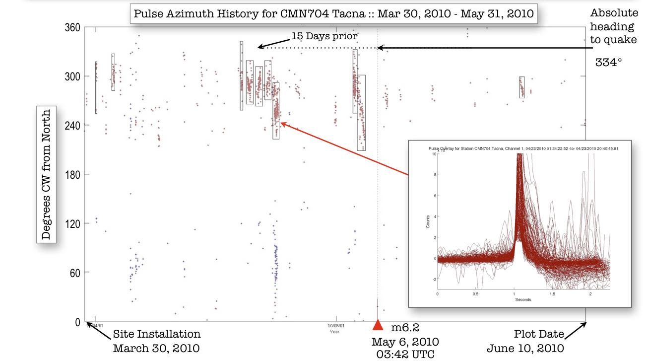
Figure1 “Azimuth clustering” of the angle of arrival of pulse energy. (quake occurred May5)
First, all the “unipolar” pulses were identified and tagged (Fig. 1 inset-pulse overlays in the lower right of the figure), Then the amplitude of each of the North-South and East-West channels were pulses used in an arctan algorithm to obtain an approximate enagle of arrival. As can be seen in the Figure 1, the pattern appears to change from a “random” angle of arrival, to one centered around 290 deg. and one around 260 deg. (+/- 30 to 60 deg.). The heading to the quake is to the “epicenter” not hypocenter.
Why don’t the pulse azimuth line up with the direction to the eventual epicenter?
The currents in the ground are not perfect conductors and have a direction of their own. In Figure 2 below, the coils are white in the distance, the vectors from the coils to the current source are yellow lines, and the current vectors at the hypocenter are blue (blue j1, j2….j5) in the foreground.
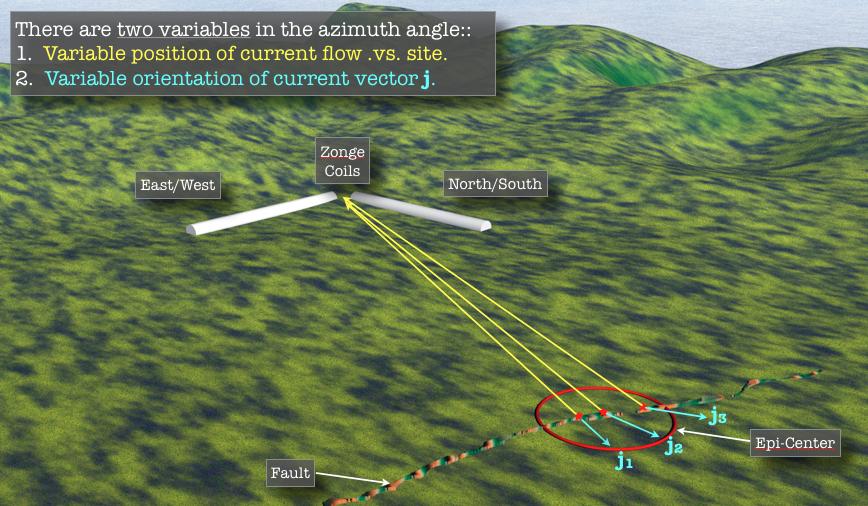
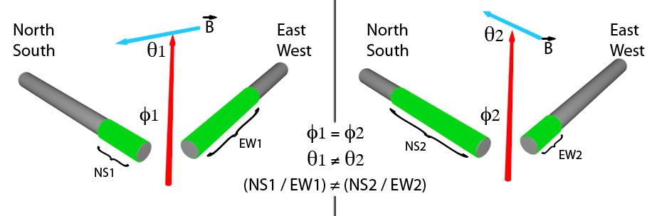
Figure 2 – Model of the Pulse Azimuth Effect. The green segments show relative projected amplitude. If phi, the angle to the location of the current flow measured referenced to the coils remains unchanged (yellow lines), but theta, the angle of the field near that current flow site changes (changing direction of the blue lines), then the ratio of energy projected on the coils, will also change.
The theory is that the currents are originating near the hypocenter, but they propagate outward from the hypocenter in different directions. Also, the hypocenter area is probably not exactly one location, but an “area along the fault”. Both of these situations would cause the apparent direction to the coils to change somewhat. The important point is that these currents seem to “cluster” near the hypocenter just before the fault ruptures.
We saw this effect in Tacna, Peru earthquake (May 5, 2010 M6.2) as well as the Oct 30, 2007 M5.4 earthquake. They also became apparent for smaller quakes (M4.5-M5) near Tacna in late 2010.
If we then combine the Pulse Count increases observed in the 2 weeks prior to medium to large earthquakes, with Pulse Azimuth Clustering, the Positive and Negative Air Conductivity changes, and the Infra Red Night Time Apparent Heating, we see a pattern of multiple effects or “discriminators” that can be used to identify the location, time and magnitude (eventually perhaps) of the future earthquake.